Photonics Research, 2019, 7 (8): 08000890, Published Online: Jul. 25, 2019
Optimal illumination scheme for isotropic quantitative differential phase contrast microscopy  Download: 719次
Figures & Tables
Fig. 1. Schematic diagram of the integral for PTF along the left–right axis in the polar coordinate system. (a) The radius ρ Q NA obj ≤ ρ ≤ 2 NA obj ρ Q 0 ≤ ρ < NA obj
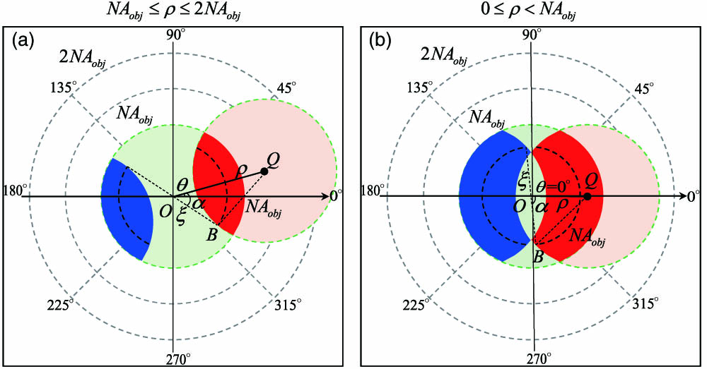
Fig. 2. PTF and C ( ρ , θ ) C ( ρ , θ ) C ( ρ , θ ) C ( ρ , θ )

Fig. 3. Simulation results with different regularization parameters under four illumination patterns. (a) Original phase image. (b) Diffraction limit phase image of DPC (2 NA obj 2 NA obj

Fig. 4. Phase reconstruction results of a phase resolution target QPT TM 2 NA obj

Fig. 5. Phase reconstruction results of HeLa cells under the optimal illumination scheme. (a) Full-field-of-view phase distribution. (b), (c) Phase maps of two selected zooms. (d) Phase results at different time points.

Fig. 6. Schematic diagram of the integral for PTF along the left–right axis illumination in the polar coordinate system. (a) The radius ρ Q NA obj ≤ ρ ≤ 2 NA obj ρ Q 0 ≤ ρ < NA obj

Fig. 7. PTF and C ( ρ , θ ) L ( ρ ) C ( ρ , θ ) C ( ρ , θ )

Fig. 8. PTF and C ( ρ , θ ) σ C ( ρ , θ ) C ( ρ , θ )

Fig. 9. PTF and C ( ρ , θ ) n C ( ρ , θ ) C ( ρ , θ )


Yao Fan, Jiasong Sun, Qian Chen, Xiangpeng Pan, Lei Tian, Chao Zuo. Optimal illumination scheme for isotropic quantitative differential phase contrast microscopy[J]. Photonics Research, 2019, 7(8): 08000890.


 PDF全文
PDF全文

